Supplement 2: Estimate different causal effects in a hypothetical RCT

Authors

Affiliations

Lukas Junker

LMU Munich

Ramona Schoedel

Charlotte Fresenius University, Munich

LMU Munich

Florian Pargent

LMU Munich

Introduction of the hypothetical RCT

In our manuscript, we introduce the following hypothetical RCT in the section Running Example for Causal Inference in Longitudinal Study Designs:

Consider a smartphone study in which participants are randomly assigned to use a specific social media app from 8 PM to 10 PM (\(t = 1\)) or not. There is no intervention afterwards, meaning that from 10 PM to midnight (\(t = 2\)), participants can decide for themselves whether to use this app, and this usage is passively recorded. We set \(a_t=1\) if the social media app was used during the time frame indexed by \(t\), while \(a_t=0\) means that the app was not used at all during \(t\). At 10 PM, participants’ rumination (\(L\)) is also measured, as it is hypothesized to be another mediator between social media usage and sleep quality. The final outcome of the study, sleep quality (\(Y\)), is measured the next morning. Figure 1 presents a DAG corresponding to this RCT. Because early social media usage was manipulated in an experiment, there are no arrows pointing into \(A_1\). In contrast, \(A_2\) can be influenced by both \(A_1\) and \(L\). The variable \(U\) represents the set of all unmeasured confounders. Note that in our example, we make the strong assumption that \(U\) is not a direct cause of \(A_2\), and we discuss this potentially implausible assumption in the manuscript section on identification.

In Supplement 1 we showed how to estimate expected potential outcomes and reproduce Table 1 in our manuscript. Here in Supplement 2, we will demonstrate in R how we can simulate and (try to) estimate different total, joint, and direct causal effects.

Demonstration in R

We will use the same DAG and data generating process as in Supplement 1, but will repeat all R code here for completeness.

Load packages

library(tidyverse)
library(dagitty)
library(brms)
library(cmdstanr)
library(tidybayes)

Specify the data generating process

Draw the DAG

Code

dag <- dagitty('dag{
  A1 -> L <- U
  A1 -> A2 <- L
  A1 -> Y <- A2
  L -> Y <- U
  A1[pos="0,2"]
  A2[pos="1,2"]
  Y[pos="1.5,1.5"]
  L[pos="0.5,1.5"]
  U[pos="1,1"]
  }')
plot(dag)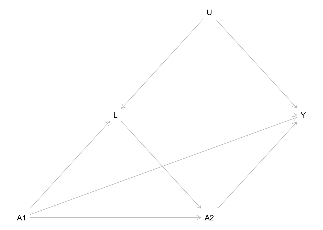

Figure 1: DAG that corresponds to an RCT with repeated measurements. \(U\) denotes unmeasured confounding, while \(L\) and \(A_2\) are measured mediators of the causal effect of \(A_1\) on the end of study outcome \(Y\). Since \(A_1\) is randomized, there are no arrows pointing into it.

Specify the functional relationships

To showcase joint effect estimation, we again simulate a scenario where \(U\) affects \(A_2\) only through measured \(L\). We discuss situations in which this assumption may be plausible in psychological research—induced by covariate-driven treatment assignment—in the latter half of the manuscript.

b_L_A1 <- 1
b_L_U <- 1
b_A2_A1 <- -3
b_A2_L <- 0.5
b_A2_U <- 0
b_Y_A1 <- -0.1
b_Y_A2 <- -3
b_Y_L <- -1
b_Y_A1A2 <- -0.5
b_Y_U <- -2


f_U <- function(){
  rnorm(n)}
f_A1 <- function(){
  rbinom(n, size = 1, prob = 0.5)}
f_L <- function(A1, U){
  rnorm(n, mean = b_L_A1 * A1 + b_L_U * U)}
f_A2 <- function(A1, L){
  rbinom(n, size = 1, prob = pnorm(b_A2_A1 * A1 + b_A2_L* L + b_A2_U * U))}
f_Y <- function(A1, A2, L, U){
  rnorm(n, mean = 10 + b_Y_A1 * A1 + b_Y_A2 * A2 + b_Y_A1A2 * A1 * A2 + b_Y_L * L +
      b_Y_U * U, sd = 0.1)}

Determine the true causal effects

We will now simulate various causal effects for our hypothetical RCT:

Total effect of A1: \(E(Y^{a_1=1}) - E(Y^{a_1=0})\)

n <- 10000000
set.seed(42)

# Y_1: Y^{a_1=1}

U <- f_U()
A1 <- rep(1, n) # intervention
L <- f_L(A1, U)
A2 <- f_A2(A1, L)
Y_1 <- f_Y(A1, A2, L, U)

# Y_0: Y^{a_1=0}

U <- f_U()
A1 <- rep(0, n) # intervention
L <- f_L(A1, U)
A2 <- f_A2(A1, L)
Y_0 <- f_Y(A1, A2, L, U)

# E(Y_1) - E(Y_0)
(total_A1 <- mean(Y_1) - mean(Y_0))

[1] 0.3257348

Joint effect “always - never”: \(E(Y^{a_1=1, a_2=1}) - E(Y^{a_1=0, a_2=0})\)

n <- 10000000
set.seed(42)

# Y_11: Y^{a_1=1, a_2=1}

U <- f_U()
A1 <- rep(1, n) # intervention
L <- f_L(A1, U)
A2 <- rep(1, n) # intervention
Y_11 <- f_Y(A1, A2, L, U)

# Y_00: Y^{a_1=0, a_2=0}

U <- f_U()
A1 <- rep(0, n) # intervention
L <- f_L(A1, U)
A2 <-  rep(0, n) # intervention
Y_00 <- f_Y(A1, A2, L, U)

# E(Y_11) - E(Y_00)
(joint_always <- mean(Y_11) - mean(Y_00))

[1] -4.600175

Joint effect “early use”: \(E(Y^{a_1=1, a_2=0}) - E(Y^{a_1=0, a_2=0})\)

n <- 10000000
set.seed(42)

# Y_10: Y^{a_1=1, a_2=0}

U <- f_U()
A1 <- rep(1, n) # intervention
L <- f_L(A1, U)
A2 <- rep(0, n) # intervention
Y_10 <- f_Y(A1, A2, L, U)

# Y_00: Y^{a_1=0, a_2=0}

U <- f_U()
A1 <- rep(0, n) # intervention
L <- f_L(A1, U)
A2 <- rep(0, n) # intervention
Y_00 <- f_Y(A1, A2, L, U)

# E(Y_10) - E(Y_00)
(joint_early <- mean(Y_10) - mean(Y_00))

[1] -1.100175

Joint effect “late use”: \(E(Y^{a_1=0, a_2=1}) - E(Y^{a_1=0, a_2=0})\)

n <- 10000000
set.seed(42)

# Y_01: Y^{a_1=0, a_2=1}

U <- f_U()
A1 <- rep(0, n) # intervention
L <- f_L(A1, U)
A2 <- rep(1, n) # intervention
Y_10 <- f_Y(A1, A2, L, U)

# Y_00: Y^{a_1=0, a_2=0}

U <- f_U()
A1 <- rep(0, n) # intervention
L <- f_L(A1, U)
A2 <- rep(0, n) # intervention
Y_00 <- f_Y(A1, A2, L, U)

# E(Y_01) - E(Y_00)
(joint_late <- mean(Y_10) - mean(Y_00))

[1] -3.000175

Direct effect “always - never”: \(E(Y^{a_1=1, L^{a_1=0}, a_2=1}) - E(Y^{a_1=0, L^{a_1=0}, a_2=0})\)

n <- 10000000
set.seed(42)

# Y_11: Y^{a_1=1, L^{a_1=0}, a_2=1}

U <- f_U()
A1 <- rep(1, n) # intervention
L <- f_L(A1 = rep(0, n), U)
A2 <- rep(1, n) # intervention
Y_10 <- f_Y(A1, A2, L, U)

# Y_00: Y^{a_1=0, L^{a_1=0}, a_2=0}

U <- f_U()
A1 <- rep(0, n) # intervention
L <-  f_L(A1, U)
A2 <-  rep(0, n) # intervention
Y_00 <- f_Y(A1, A2, L, U)

# E(Y_10) - E(Y_00)
(direct_always <- mean(Y_10) - mean(Y_00))

[1] -3.600175

Direct effect “early use”: \(E(Y^{a_1=1, L^{a_1=0}, a_2=0}) - E(Y^{a_1=0, L^{a_1=0}, a_2=0})\)

n <- 10000000
set.seed(42)

# Y_10: Y^{a_1=1, L^{a_1=0}, a_2=0}

U <- f_U()
A1 <- rep(1, n) # intervention
L <- f_L(A1 = rep(0, n), U)
A2 <- rep(0, n) # intervention
Y_10 <- f_Y(A1, A2, L, U)

# Y_00: Y^{a_1=0, L^{a_1=0}, a_2=0}

U <- f_U()
A1 <- rep(0, n) # intervention
L <-  f_L(A1, U)
A2 <-  rep(0, n) # intervention
Y_00 <- f_Y(A1, A2, L, U)

# E(Y_10) - E(Y_00)
(direct_early <- mean(Y_10) - mean(Y_00))

[1] -0.1001748

Direct effect “late use”: \(E(Y^{a_1=0, L^{a_1=0}, a_2=1}) - E(Y^{a_1=0, L^{a_1=0}, a_2=0})\)

n <- 10000000
set.seed(42)

# Y_01: Y^{a_1=0, L^{a_1=0}, a_2=1}

U <- f_U()
A1 <- rep(0, n) # intervention
L <- f_L(A1, U)
A2 <- rep(1, n) # intervention
Y_01 <- f_Y(A1, A2, L, U)

# Y_00: Y^{a_1=0, L^{a_1=0}, a_2=0}

U <- f_U()
A1 <- rep(0, n) # intervention
L <-  f_L(A1, U)
A2 <-  rep(0, n) # intervention
Y_00 <- f_Y(A1, A2, L, U)

# E(Y_01) - E(Y_00)
(direct_late <- mean(Y_01) - mean(Y_00))

[1] -3.000175

Direct effect of A1: \(E(Y^{a_1=1, L^{a_1=0}, A_2^{a_1=0, L^{a_1=0}}}) - E(Y^{a_1=0, L^{a_1=0}, A_2^{a_1=0, L^{a_1=0}}})\)

n <- 10000000
set.seed(42)

# Y_1: Y^{a_1=1, L^{a_1=0}, A_2^{a_1=0, L^{a_1=0}}}

U <- f_U()
A1 <- rep(1, n) # intervention
L <- f_L(A1 = rep(0, n), U)
A2 <- f_A2(A1 = rep(0, n), L)
Y_1 <- f_Y(A1, A2, L, U)

# Y_0: Y^{a_1=0, L^{a_1=0}, A_2^{a_1=0, L^{a_1=0}}}

U <- f_U()
A1 <- rep(0, n) # intervention
L <-  f_L(A1, U)
A2 <- f_A2(A1, L)
Y_0 <- f_Y(A1, A2, L, U)

# E(Y_1) - E(Y_0)
(direct_A1 <- mean(Y_1) - mean(Y_0))

[1] -0.351657

Simulate a sample dataset

n <- 2000
set.seed(42)

U <- f_U()
A1 <- f_A1()
L <- f_L(A1, U)
A2 <- f_A2(A1, L)
Y <- f_Y(A1, A2, L, U)

dat <- data.frame(A1, A2, L, Y)

Fit statistical models with brms

In the hypothetical RCT, there was no randomization at \(t = 2\). However, we can still estimate causal effects using our knowledge of the DAG. Causal effects can be retrieved under the assumptions of consistency, exchangeability, and positivity.

Different statistical models are required to estimate various total, joint, and direct effects. To estimate the joint effect, we ensure exchangeability by leveraging the property that, given \(L\) and \(A_1\), \(A_2\) is independent of \(U\): \(P(A_2 = a_2 | A_1, L, U) = P(A_2 = a_2 | A_1, L)\).

set.seed(42)
fit_total <- brm(Y ~ A1,
  data = dat, chains = 4, cores = 4, backend = "cmdstanr", refresh = 0)

Running MCMC with 4 parallel chains...

Chain 1 finished in 0.1 seconds.
Chain 2 finished in 0.1 seconds.
Chain 3 finished in 0.1 seconds.
Chain 4 finished in 0.1 seconds.

All 4 chains finished successfully.
Mean chain execution time: 0.1 seconds.
Total execution time: 0.2 seconds.

summary(fit_total)

 Family: gaussian 
  Links: mu = identity; sigma = identity 
Formula: Y ~ A1 
   Data: dat (Number of observations: 2000) 
  Draws: 4 chains, each with iter = 2000; warmup = 1000; thin = 1;
         total post-warmup draws = 4000

Regression Coefficients:
          Estimate Est.Error l-95% CI u-95% CI Rhat Bulk_ESS Tail_ESS
Intercept     8.62      0.12     8.38     8.85 1.00     3669     2699
A1            0.22      0.16    -0.10     0.55 1.00     4111     2991

Further Distributional Parameters:
      Estimate Est.Error l-95% CI u-95% CI Rhat Bulk_ESS Tail_ESS
sigma     3.67      0.06     3.56     3.79 1.00     4181     3032

Draws were sampled using sample(hmc). For each parameter, Bulk_ESS
and Tail_ESS are effective sample size measures, and Rhat is the potential
scale reduction factor on split chains (at convergence, Rhat = 1).

set.seed(42)
bf_L <- bf(L ~ A1)
bf_Y <- bf(Y ~ A1 + A2 + A1:A2 + L)
fit_joint <- brm(bf_L + bf_Y + set_rescor(FALSE),
  data = dat, chains = 4, cores = 4, backend = "cmdstanr", refresh = 0)

Running MCMC with 4 parallel chains...

Chain 1 finished in 0.2 seconds.
Chain 2 finished in 0.2 seconds.
Chain 3 finished in 0.2 seconds.
Chain 4 finished in 0.2 seconds.

All 4 chains finished successfully.
Mean chain execution time: 0.2 seconds.
Total execution time: 0.3 seconds.

summary(fit_joint)

 Family: MV(gaussian, gaussian) 
  Links: mu = identity; sigma = identity
         mu = identity; sigma = identity 
Formula: L ~ A1 
         Y ~ A1 + A2 + A1:A2 + L 
   Data: dat (Number of observations: 2000) 
  Draws: 4 chains, each with iter = 2000; warmup = 1000; thin = 1;
         total post-warmup draws = 4000

Regression Coefficients:
            Estimate Est.Error l-95% CI u-95% CI Rhat Bulk_ESS Tail_ESS
L_Intercept    -0.06      0.04    -0.15     0.03 1.00     6379     3045
Y_Intercept     9.94      0.07     9.81    10.07 1.00     3419     2984
L_A1            1.04      0.06     0.92     1.17 1.00     6719     3107
Y_A1            0.95      0.09     0.78     1.12 1.00     2967     2975
Y_A2           -2.92      0.10    -3.11    -2.74 1.00     3263     3119
Y_L            -2.00      0.02    -2.05    -1.95 1.00     4845     3227
Y_A1:A2        -0.25      0.27    -0.78     0.29 1.00     5005     3428

Further Distributional Parameters:
        Estimate Est.Error l-95% CI u-95% CI Rhat Bulk_ESS Tail_ESS
sigma_L     1.42      0.02     1.38     1.47 1.00     7518     2878
sigma_Y     1.41      0.02     1.37     1.45 1.00     7069     3101

Draws were sampled using sample(hmc). For each parameter, Bulk_ESS
and Tail_ESS are effective sample size measures, and Rhat is the potential
scale reduction factor on split chains (at convergence, Rhat = 1).

set.seed(42)
bf_L <- bf(L ~ A1)
bf_A2 <- bf(A2 ~ A1 + L, family = bernoulli(link = probit))
bf_Y <- bf(Y ~ A1 + A2 + A1:A2 + L)
fit_direct <- brm(bf_L + bf_A2 + bf_Y + set_rescor(FALSE),
  data = dat, chains = 4, cores = 4, backend = "cmdstanr", refresh = 0)

Running MCMC with 4 parallel chains...

Chain 1 finished in 2.3 seconds.
Chain 2 finished in 2.4 seconds.
Chain 4 finished in 2.4 seconds.
Chain 3 finished in 2.5 seconds.

All 4 chains finished successfully.
Mean chain execution time: 2.4 seconds.
Total execution time: 2.6 seconds.

summary(fit_direct)

 Family: MV(gaussian, bernoulli, gaussian) 
  Links: mu = identity; sigma = identity
         mu = probit
         mu = identity; sigma = identity 
Formula: L ~ A1 
         A2 ~ A1 + L 
         Y ~ A1 + A2 + A1:A2 + L 
   Data: dat (Number of observations: 2000) 
  Draws: 4 chains, each with iter = 2000; warmup = 1000; thin = 1;
         total post-warmup draws = 4000

Regression Coefficients:
             Estimate Est.Error l-95% CI u-95% CI Rhat Bulk_ESS Tail_ESS
L_Intercept     -0.06      0.05    -0.15     0.03 1.00     5199     3225
A2_Intercept     0.00      0.05    -0.09     0.09 1.00     5676     2987
Y_Intercept      9.94      0.07     9.82    10.07 1.00     2978     2936
L_A1             1.04      0.06     0.92     1.17 1.00     5424     3241
A2_A1           -2.83      0.13    -3.08    -2.58 1.00     2437     2966
A2_L             0.50      0.03     0.44     0.57 1.00     3249     3052
Y_A1             0.95      0.09     0.77     1.12 1.00     2403     2728
Y_A2            -2.92      0.10    -3.11    -2.73 1.00     2937     2915
Y_L             -2.00      0.02    -2.05    -1.95 1.00     3521     3206
Y_A1:A2         -0.25      0.29    -0.84     0.31 1.00     4778     3432

Further Distributional Parameters:
        Estimate Est.Error l-95% CI u-95% CI Rhat Bulk_ESS Tail_ESS
sigma_L     1.42      0.02     1.38     1.47 1.00     4393     2804
sigma_Y     1.41      0.02     1.36     1.46 1.00     5205     3063

Draws were sampled using sample(hmc). For each parameter, Bulk_ESS
and Tail_ESS are effective sample size measures, and Rhat is the potential
scale reduction factor on split chains (at convergence, Rhat = 1).

Estimate the causal effects

params_total <- tidy_draws(fit_total)
params_joint <- tidy_draws(fit_joint)
params_direct <- tidy_draws(fit_direct)
N <- 10000

# total effect A1
total_A1_est <- params_total |> 
  group_by(.draw) |>
  mutate(
    E_Y_1 = {
      a1 <- rep(1, N)
      y <- rnorm(N, b_Intercept + b_A1 * a1, sd = sigma)
      mean(y)},
    E_Y_0 = {
      a1 <- rep(0, N)
      y <- rnorm(N, b_Intercept + b_A1 * a1, sd = sigma)
      mean(y)}) |>
  mutate(E_Y_diff = E_Y_1 - E_Y_0) |>
  ungroup() |> select(E_Y_diff) |>
  summarise_draws()

# joint effect always - never
joint_always_est <- params_joint |> 
  group_by(.draw) |>
  mutate(
    E_Y_11 = {
      a1 <- rep(1, N)
      l <- rnorm(N, b_L_Intercept + b_L_A1 * a1, sd = sigma_L)
      a2 <- rep(1, N)
      y <- rnorm(N, b_Y_Intercept + b_Y_A1 * a1 + b_Y_A2 * a2 + `b_Y_A1:A2` * a1 * a2 +
          b_Y_L * l, sd = sigma_Y)
      mean(y)},
    E_Y_00 = {
      a1 <- rep(0, N)
      l <- rnorm(N, b_L_Intercept + b_L_A1 * a1, sd = sigma_L)
      a2 <- rep(0, N)
      y <- rnorm(N, b_Y_Intercept + b_Y_A1 * a1 + b_Y_A2 * a2 + `b_Y_A1:A2` * a1 * a2 +
          b_Y_L * l, sd = sigma_Y)
      mean(y)}) |>
  mutate(E_Y_diff = E_Y_11 - E_Y_00) |>
  ungroup() |> select(E_Y_diff) |>
  summarise_draws()

# joint effect early use
joint_early_est <- params_joint |> 
  group_by(.draw) |>
  mutate(
    E_Y_10 = {
      a1 <- rep(1, N)
      l <- rnorm(N, b_L_Intercept + b_L_A1 * a1, sd = sigma_L)
      a2 <- rep(0, N)
      y <- rnorm(N, b_Y_Intercept + b_Y_A1 * a1 + b_Y_A2 * a2 + `b_Y_A1:A2` * a1 * a2 +
          b_Y_L * l, sd = sigma_Y)
      mean(y)},
    E_Y_00 = {
      a1 <- rep(0, N)
      l <- rnorm(N, b_L_Intercept + b_L_A1 * a1, sd = sigma_L)
      a2 <- rep(0, N)
      y <- rnorm(N, b_Y_Intercept + b_Y_A1 * a1 + b_Y_A2 * a2 + `b_Y_A1:A2` * a1 * a2 +
          b_Y_L * l, sd = sigma_Y)
      mean(y)}) |>
  mutate(E_Y_diff = E_Y_10 - E_Y_00) |>
  ungroup() |> select(E_Y_diff) |>
  summarise_draws()

# joint effect late use
joint_late_est <- params_joint |> 
  group_by(.draw) |>
  mutate(
    E_Y_01 = {
      a1 <- rep(0, N)
      l <- rnorm(N, b_L_Intercept + b_L_A1 * a1, sd = sigma_L)
      a2 <- rep(1, N)
      y <- rnorm(N, b_Y_Intercept + b_Y_A1 * a1 + b_Y_A2 * a2 + `b_Y_A1:A2` * a1 * a2 +
          b_Y_L * l, sd = sigma_Y)
      mean(y)},
    E_Y_00 = {
      a1 <- rep(0, N)
      l <- rnorm(N, b_L_Intercept + b_L_A1 * a1, sd = sigma_L)
      a2 <- rep(0, N)
      y <- rnorm(N, b_Y_Intercept + b_Y_A1 * a1 + b_Y_A2 * a2 + `b_Y_A1:A2` * a1 * a2 +
          b_Y_L * l, sd = sigma_Y)
      mean(y)}) |>
  mutate(E_Y_diff = E_Y_01 - E_Y_00) |>
  ungroup() |> select(E_Y_diff) |>
  summarise_draws()

# direct effect always - never
direct_always_est <- params_joint |> 
  group_by(.draw) |>
  mutate(
    E_Y_11 = {
      a1 <- rep(1, N)
      a1_0 <- rep(0, N)
      l <- rnorm(N, b_L_Intercept + b_L_A1 * a1_0, sd = sigma_L)
      a2 <- rep(1, N)
      y <- rnorm(N, b_Y_Intercept + b_Y_A1 * a1 + b_Y_A2 * a2 + `b_Y_A1:A2` * a1 * a2 +
          b_Y_L * l, sd = sigma_Y)
      mean(y)},
    E_Y_00 = {
      a1 <- rep(0, N)
      l <- rnorm(N, b_L_Intercept + b_L_A1 * a1, sd = sigma_L)
      a2 <- rep(0, N)
      y <- rnorm(N, b_Y_Intercept + b_Y_A1 * a1 + b_Y_A2 * a2 + `b_Y_A1:A2` * a1 * a2 +
          b_Y_L * l, sd = sigma_Y)
      mean(y)}) |>
  mutate(E_Y_diff = E_Y_11 - E_Y_00) |>
  ungroup() |> select(E_Y_diff) |>
  summarise_draws()

# direct effect early use
direct_early_est <- params_joint |> 
  group_by(.draw) |>
  mutate(
    E_Y_10 = {
      a1 <- rep(1, N)
      a1_0 <- rep(0, N)
      l <- rnorm(N, b_L_Intercept + b_L_A1 * a1_0, sd = sigma_L)
      a2 <- rep(0, N)
      y <- rnorm(N, b_Y_Intercept + b_Y_A1 * a1 + b_Y_A2 * a2 + `b_Y_A1:A2` * a1 * a2 +
          b_Y_L * l, sd = sigma_Y)
      mean(y)},
    E_Y_00 = {
      a1 <- rep(0, N)
      l <- rnorm(N, b_L_Intercept + b_L_A1 * a1, sd = sigma_L)
      a2 <- rep(0, N)
      y <- rnorm(N, b_Y_Intercept + b_Y_A1 * a1 + b_Y_A2 * a2 + `b_Y_A1:A2` * a1 * a2 +
          b_Y_L * l, sd = sigma_Y)
      mean(y)}) |>
  mutate(E_Y_diff = E_Y_10 - E_Y_00) |>
  ungroup() |> select(E_Y_diff) |>
  summarise_draws()

# direct effect late use
direct_late_est <- params_joint |> 
  group_by(.draw) |>
  mutate(
    E_Y_01 = {
      a1 <- rep(0, N)
      l <- rnorm(N, b_L_Intercept + b_L_A1 * a1, sd = sigma_L)
      a2 <- rep(1, N)
      y <- rnorm(N, b_Y_Intercept + b_Y_A1 * a1 + b_Y_A2 * a2 + `b_Y_A1:A2` * a1 * a2 +
          b_Y_L * l, sd = sigma_Y)
      mean(y)},
    E_Y_00 = {
      a1 <- rep(0, N)
      l <- rnorm(N, b_L_Intercept + b_L_A1 * a1, sd = sigma_L)
      a2 <- rep(0, N)
      y <- rnorm(N, b_Y_Intercept + b_Y_A1 * a1 + b_Y_A2 * a2 + `b_Y_A1:A2` * a1 * a2 +
          b_Y_L * l, sd = sigma_Y)
      mean(y)}) |>
  mutate(E_Y_diff = E_Y_01 - E_Y_00) |>
  ungroup() |> select(E_Y_diff) |>
  summarise_draws()

# direct effect A1
direct_A1_est <- params_direct |> 
  group_by(.draw) |>
  mutate(
    E_Y_1 = {
      a1 <- rep(1, N)
      a1_0 <- rep(0, N)
      l <- rnorm(N, b_L_Intercept + b_L_A1 * a1_0, sd = sigma_L)
      a2 <- rbinom(N, size = 1, prob = pnorm(b_A2_Intercept + b_A2_A1 * a1_0 + b_A2_L * l))
      y <- rnorm(N, b_Y_Intercept + b_Y_A1 * a1 + b_Y_A2 * a2 + `b_Y_A1:A2` * a1 * a2 +
          b_Y_L * l, sd = sigma_Y)
      mean(y)},
    E_Y_0 = {
      a1 <- rep(0, N)
      l <- rnorm(N, b_L_Intercept + b_L_A1 * a1, sd = sigma_L)
      a2 <- rbinom(N, size = 1, prob = pnorm(b_A2_Intercept + b_A2_A1 * a1 + b_A2_L * l))
      y <- rnorm(N, b_Y_Intercept + b_Y_A1 * a1 + b_Y_A2 * a2 + `b_Y_A1:A2` * a1 * a2 +
          b_Y_L * l, sd = sigma_Y)
      mean(y)}) |>
  mutate(E_Y_diff = E_Y_1 - E_Y_0) |>
  ungroup() |> select(E_Y_diff) |>
  summarise_draws()

Compare the true causal effects with their empirical estimates

Code

table <- tribble(
 ~"causal effect"               ,~"true effect" ,~"estimate (med)"        ,~"ci (q2.5)"           ,~"ci (q97.5)",
  "total effect A1"             , total_A1      , total_A1_est$median     , total_A1_est$q5     , total_A1_est$q95     ,
  "joint effect always - never" , joint_always  , joint_always_est$median , joint_always_est$q5 , joint_always_est$q95 ,
  "joint effect early use"      , joint_early   , joint_early_est$median  , joint_early_est$q5  , joint_early_est$q95  ,
  "joint effect late use"       , joint_late    , joint_late_est$median   , joint_late_est$q5   , joint_late_est$q95   ,
  "direct effect always - never", direct_always , direct_always_est$median, direct_always_est$q5, direct_always_est$q95,
  "direct effect early use"     , direct_early  , direct_early_est$median , direct_early_est$q5 , direct_early_est$q95 ,
  "direct effect late use"      , direct_late   , direct_late_est$median  , direct_late_est$q5  , direct_late_est$q95  ,
  "direct effect A1"            , direct_A1     , direct_A1_est$median    , direct_A1_est$q5    , direct_A1_est$q95    ,

)
knitr::kable(table)

causal effect	true effect	estimate (med)	ci (q2.5)	ci (q97.5)
total effect A1	0.3257348	0.2219661	-0.0601195	0.5047605
joint effect always - never	-4.6001748	-4.3157444	-4.8158236	-3.8104642
joint effect early use	-1.1001748	-1.1365596	-1.3962049	-0.8839994
joint effect late use	-3.0001748	-2.9251223	-3.0979420	-2.7480792
direct effect always - never	-3.6001748	-2.2275346	-2.6955974	-1.7778516
direct effect early use	-0.1001748	0.9491820	0.7884349	1.1102144
direct effect late use	-3.0001748	-2.9262275	-3.0978062	-2.7513584
direct effect A1	-0.3516570	0.8259555	0.5603612	1.0852940

Note that the total and joint effects are estimated without bias, while the direct effects are biased because of the unobserved confounder \(U\) (except for the direct effect of “late use”, which for our data generating process is equal to the joint effect of “late use”).

Reuse

CC BY 4.0

Citation

BibTeX citation:

@article{junker2025,
  author = {Junker, Lukas and Schoedel, Ramona and Pargent, Florian},
  title = {Towards a {Clearer} {Understanding} of {Causal} {Estimands:}
    {The} {Importance} of {Joint} {Effects} in {Longitudinal} {Designs}
    with {Time-Varying} {Treatments.}},
  journal = {PsyArXiv},
  date = {2025},
  url = {https://FlorianPargent.github.io/joint_effects_ampps/supplement_2.html},
  doi = {10.31234/osf.io/zmh5a},
  langid = {en}
}

For attribution, please cite this work as:

Junker, L., Schoedel, R., & Pargent, F. (2025). Towards a Clearer Understanding of Causal Estimands: The Importance of Joint Effects in Longitudinal Designs with Time-Varying Treatments. PsyArXiv. https://doi.org/10.31234/osf.io/zmh5a